Topic modelling with BERTopic and non negative matrix factorisation

Topic modelling is a very common task in natural language processing which involves finding topics within a large corpus of text. It’s also an area with a lot of academic development, so new methods are emerging regularly. Two of the most popular current methods for finding these topics are BERTopic and non-negative matrix factorisation (NMF). I have been playing with both of these methods and outline some things I’ve learned in weighing up the most appropriate method below. I also include a tutorial of NMF in Python below.

BERTopic

This is the most widely used method in a variety of sectors at the moment, and tutorials are available from the developer, Maarten Grootendorst, and others. Having used BERTopic, I have learned the following:

• BERTopic chooses the optimum number of topics, saving the user from having to choose themselves. You can also choose the number of topics yourself or merge topics
• The number of outliers can be high. In the first tutorial above using academic abstracts from the arXiv repository, 49% of the abstracts were classified as outliers. The percentage of outliers can be tweaked using the min_cluster_size and min_samples parameters but in my experience I could only reduce this to about 30%. This may or may not be suitable in your particular use case
• Results are better when pre-processing is applied. Pre-processing doesn’t seem to be necessary for BERTopic according to the documentation but I found it performed better when the input text was cleaned, and in particular when stop words were removed.

NMF

NMF is primarily a dimension reduction technique which can be implemented on documents. In my experience it has performed reasonably well. I have learned that:

• You need to set the number of topics as an input parameter. This inevitably involves guessing or manually testing the number of different topics and observing which appears best
• There are no outliers identified as part of the process. Although I wouldn’t want a high percentage of outliers in a corpus, intuitively we might expect at least some. Each document is given a score as to how well it is associated with each of the topics, so some assessment of a cut-off for these scores might be performed to “create” some outliers
• Pre-processing is required for this method.

NMF tutorial in Python

Below I outline how I’ve run this method on the 20 newsgroups dataset, a collection of around 18,000 newsgroup posts in 20 categories.

First of all we need to import the necessary Python libraries

import pandas as pd
from sklearn.datasets import fetch_20newsgroups
from sklearn.feature_extraction.text import TfidfVectorizer
from sklearn.decomposition import NMF
import seaborn as sns
import matplotlib.pyplot as plt

We also need to import the training subset of the 20 newsgroups dataset

data = fetch_20newsgroups(subset='train', remove=('headers', 'footers', 'quotes'))
docs = data['data']
targets = data['target']
target_names = data['target_names']
classes = [data['target_names'][i] for i in data['target']]

NMF takes numbers (rather than raw text) as an input so we need to convert our dataset of words to a collection of numbers. To do this we use Term Frequency – Inverse Document Frequency (tf-idf), which reflects how important a word is to a document. So a word such as “hockey” might score highly as it is relatively unique to a document but a word common to many documents such as “and” would have a low score. The code also removes very common words (stop words), words occurring in less than three documents or in more than 95% of documents.

tfidf_vectorizer = TfidfVectorizer(max_df=0.95, min_df=3, stop_words="english")
tfidf = tfidf_vectorizer.fit_transform(docs)

We can then run and fit the NMF model. The n_components parameter states how many topics we would like the documents to be grouped into and I have chosen 100 initially.

model = NMF(
    n_components=100,
    random_state=1,
    init="random",
    beta_loss="kullback-leibler",
    solver="mu",
    max_iter=1000,
    alpha=0.00005,
    l1_ratio=0.5
)

W = model.fit_transform(tfidf)
H = model.components_

We then need to wrangle the output data into a suitable format. For example, by putting the results of the model into a pandas dataframe and getting the topic number to which each document is most highly associated.

nmf_features = pd.DataFrame(W)
components_df = pd.DataFrame(H, columns=tfidf_vectorizer.get_feature_names())
nmf_features['Topic_number'] = nmf_features.idxmax(axis=1)

While it is useful to have a topic number, it is more intuitive to name the topics. Helpfully, each topic has a value attached to each word in the corpus, so we can use the top three words with the highest values to name each topic.

topic_names_list = []
for topic in range(components_df.shape[0]):
    tmp = components_df.iloc[topic]
    temp = tmp.nlargest(3)
    topic_name = " ".join(temp.index.tolist())
    topic_names_list.append(topic_name)

Finally we’re able to wrangle these topic names from NMF into the same dataframe as the categories from the 20 newsgroups dataset.

components_df['Topic_name'] = topic_names_list
components_df['Topic_number'] = components_df.index.tolist()

joined_df = pd.concat([pd.Series(docs), pd.Series(classes), nmf_features['Topic_number']], axis=1)
joined_df.columns = ['Docs', 'Classes', 'Topic_number']
joined_df = pd.merge(joined_df, components_df[['Topic_number', 'Topic_name']], on='Topic_number', how='inner')

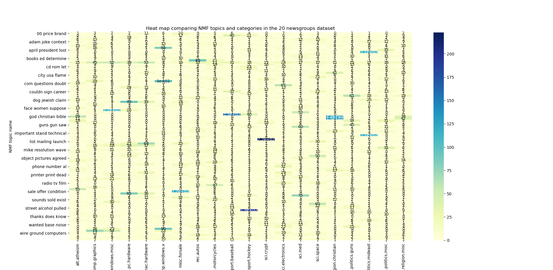
This enables us to create a heat map of the NMF topics against the categories. Not all of the names of the 100 topics are visible on the y axis.

pivot_df = pd.crosstab(index=joined_df['Topic_name'], columns=joined_df['Classes'])

ax = sns.heatmap(pivot_df, annot=True, cmap="YlGnBu")\
    .set(title='Heat map comparing NMF topics and categories in the 20 newsgroups dataset',
         xlabel='Categories', ylabel='NMF topic name')
plt.show()

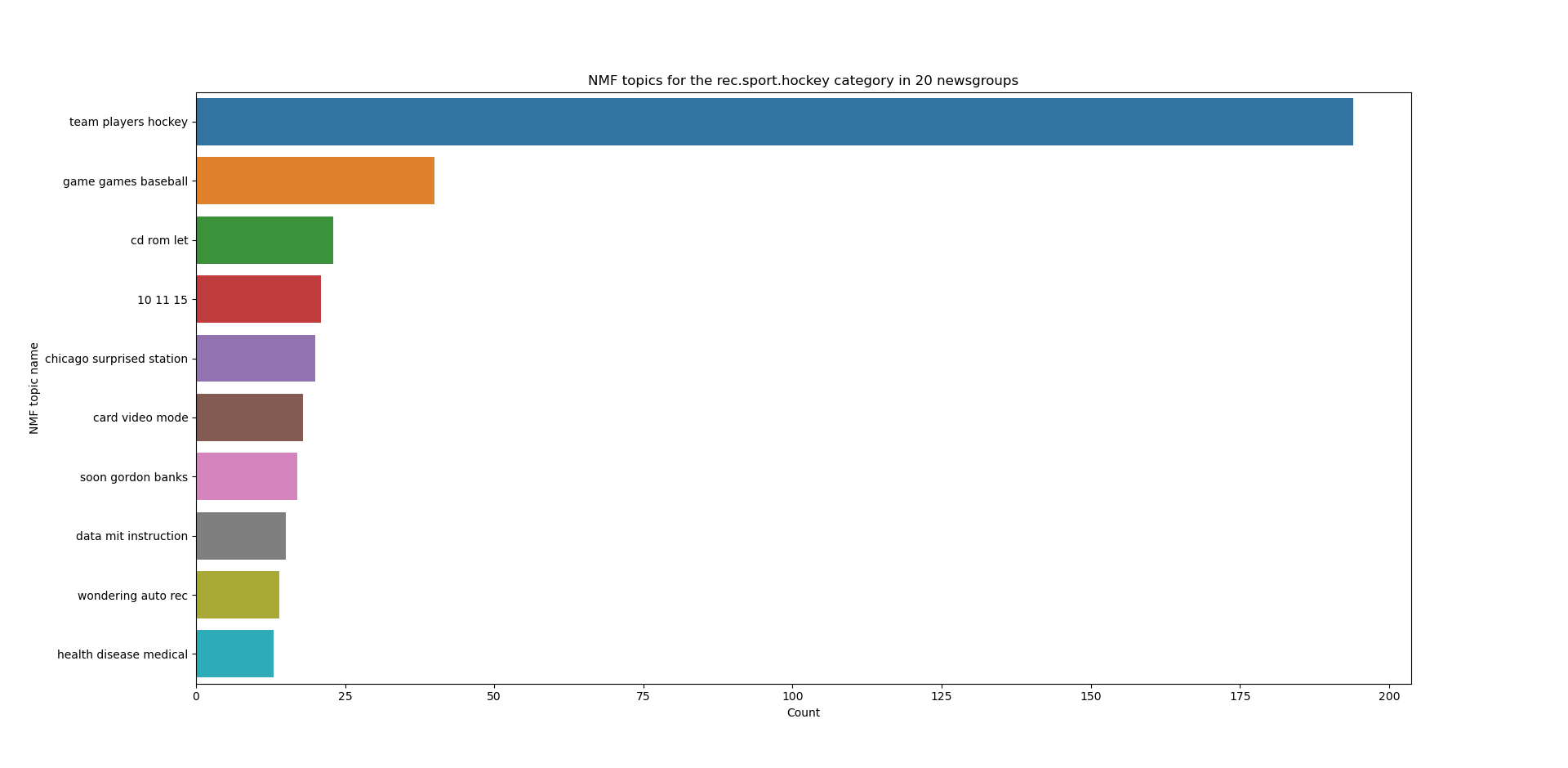
We can also extract particular categories from the 20 newsgroups dataset. For example the rec.sport.hockey category is strongly associated with the “team players hockey” NMF topic. This bar plot also highlights that more pre-processing should be done on the input text since “10 11 15” isn’t exactly a meaningful topic name!

hockey = pivot_df['rec.sport.hockey'].sort_values(ascending=False).head(10)
ax2 = sns.barplot(x=hockey, y=hockey.index)\
    .set(title='NMF topics for the rec.sport.hockey category in 20 newsgroups', xlabel='Count', ylabel='NMF topic name')
plt.show()

Summary

I’ve been playing with BERTopic and NMF for topic modelling on a corpus of text. Although very popular, the high percentage of outliers produced using BERTopic can be restrictive depending on your use case. Therefore I’ve also looked at NMF and have outlined a tutorial of how to apply this to the 20 newsgroups dataset.

The code above is available on Github. I always welcome comments or suggestions for improvements, and am keen to hear others’ experience of topic modelling techniques.